Machine Learning Tutorial (V) Naive Bayes and Text Classification

Bayes Rule in A1 (from Lec04)

• Recall \(E\) in MAP:
  • \(E(\tilde{w}) = L(\tilde{w}) + \frac{\lambda}{2}\tilde{w}^T\tilde{w}\)
• convert \(E\) back to probabilities by taking \(exp(-E)\):
  • \(exp(-E(\tilde{w})) = exp(-L(\tilde{w}) - \frac{\lambda}{2}\tilde{w}^T\tilde{w})\)
    \(= exp(-L(\tilde{w}))exp(-\frac{\lambda}{2}\tilde{w}^T\tilde{w})\)
    \(= \Pi_{i=1}^N P(t_i|x_i)exp(-\frac{\lambda}{2}\tilde{w}^T\tilde{w})\)

Bayes Rule in A1 (from Lec04)

• \(exp(-\frac{\lambda}{2}\tilde{w}^T\tilde{w})\) is proportional to a Gaussian probability density function (PDF):
• We can write this as \(p(\tilde{w}) \propto exp(-\frac{\lambda}{2}\tilde{w}^T\tilde{w})\)
• Minimizing \(E\) is equivalent to maximzing:
  • \(\Pi_{i=1}^N P(t_i|x_i)p(\tilde{w})\)

Bayes Rule in A1 (from Lec04)

• Take a look back at Baye's rule
  • \(p(\theta|D) = \frac{p(D|\theta)p(\theta)}{p(D)} \propto p(D|\theta)p(\theta)\)
• prior \((p(\theta))\): how likely \(\theta\) is before observing data.
• likelihood \((p(D|\theta))\): how likely the data set \(D\) is if the model parameter is \(\theta\).
• posterior \((p(\theta|D))\): how likely \(\theta\) is after observing the data set \(D\).
• Estimating the \(\theta\) (learning the model) by maximizing the posterior distribution is called maximum a posteriori (MAP) estimation.

Positive or negative movie review?[Dan Jurafsky]

• Unbelievably disappointing.
• This is the greatest screwball comedy ever filmed.
• It was pathetic. The worst part about it was the boxing scenes.

Classification Methods: Supervised Machine Learning

• Input:
  • a document \(d\).
  • a fixed set of classes \(C = {c_1, c_2,\ldots, c_j}\)
  • a training set of \(m\) hand-labeled documents \((d_1,c_1),\ldots,(d_m,c_m)\)
• Output:
  • a learned classifier \(\gamma: d \rightarrow c\)

The Bag of words model

• Idea: Represent a text document as a feature vector in order to use machine learning methods.
• vocabulary: the set of all different feature words that occur in training set, with a count of how it occurs.
  • ignore the order
  • occurance is independent (naive Bayes): "hello" tends to be followed by a "world"

Example of Bag of words model

• Documents:
  • D1: "Unbelievably disappointing."
  • D2: "This is the greatest screwball comedy ever filmed."
  • D3: "It was pathetic. The worst part about it was the boxing scenes."
  • D4: "Greatest film ever."
• Vocabulary
  • V = {disappointing: 1, greatest: 2, pathetic: 1, worst: 1}

A Toy Example [Sebastian Raschka]

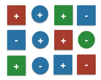
• (Training) Dataset
  • 12 samples, 2 different classes +,-.
  • 2 features: color, geometrical shape.
• Denote
  • \(c_j\) be class labels: \(c_j=+\) for +, \(c_j=-\) for -.
  • \(x_j\) be the 2-dimensional feature vectors: \(x_j = [x_{j1} x_{j2}], x_{j1} \in \{blue, green, red, yellow\}, x_{j2} \in \{circle, square\}\)

Classify a new sample

• New Sample
  • features \(x=[blue, square]\)
  • class? (ground truth: +)
• decision rule
  • (MAP) \(P(c=+ | x=[blue, square]) \ge P(c=- | x=[blue, square]) ? + : -;\)

Classify a new sample

• computing
  • (prior) \(P(+) = \frac{7}{12} = 0.58, P(-) = \frac{5}{12} = 0.42\)
  • (likelihood, +) \(P(x | +) = P(blue | +) \cdot P(square | +) = \frac{3}{7} \cdot \frac{5}{7} = 0.31\) (i.i.d.)
  • (likelihood, -) \(P(x | -) = P(blue | -) \cdot P(square | -) = \frac{3}{5} \cdot \frac{3}{5} = 0.36\) (i.i.d.)
  • (posterior, + ) \(P( + | x) \propto P(x | + ) \cdot P(+) = 0.31 \cdot 0.58 = 0.18\)
  • (posterior, -) \(P(- | x) \propto P(x | -) \cdot P(-) = 0.36 \cdot 0.42 = 0.15\)

Classify a new sample

• computing
  • (prior) \(P(+) = \frac{7}{12} = 0.58, P(-) = \frac{5}{12} = 0.42\)
  • (likelihood, +) \(P(x | +) = P(blue | +) \cdot P(square | +) = \frac{3}{7} \cdot \frac{5}{7} = 0.31\) (i.i.d.)
  • (likelihood, -) \(P(x | -) = P(blue | -) \cdot P(square | -) = \frac{3}{5} \cdot \frac{3}{5} = 0.36\) (i.i.d.)
  • (posterior, + ) \(P( + | x) \propto P(x | + ) \cdot P(+) = 0.31 \cdot 0.58 = 0.18\)
  • (posterior, -) \(P(- | x) \propto P(x | -) \cdot P(-) = 0.36 \cdot 0.42 = 0.15\)
• on dropping \(p(x)\)
  • \(p(x)\) is called evidence
  • no effect on the final result
• classification
  • \(P(+ | x) \ge P(- | x)\), so classfied as +.

A trickier case

• New Sample
  • features \(x=[yellow, square]\)
  • likelihood \(P(x | +) = P(yellow | +) \cdot P(square | +) = 0 \cdot \frac{5}{7} = 0\) ?
• Laplace (add-1) smoothing
  • \(\hat{P}(x_i | c)\)
  • \(= \frac{count(x_i, c) + 1}{\Sigma_{x \in V}(count(x, c) + 1)}\)
  • \(= \frac{count(x_i, c) + 1}{\Sigma_{x \in V}count(x, c) + |V|}\)

Summarize and apply to Text Classification

• (training set) feature extraction (bag of words)
• Naive Bayes and Language Modeling
  • prior (class)
  • likelihood (i.i.d., laplace smoothing)
  • drop the evidence term
  • compute posterior
  • apply decision rule

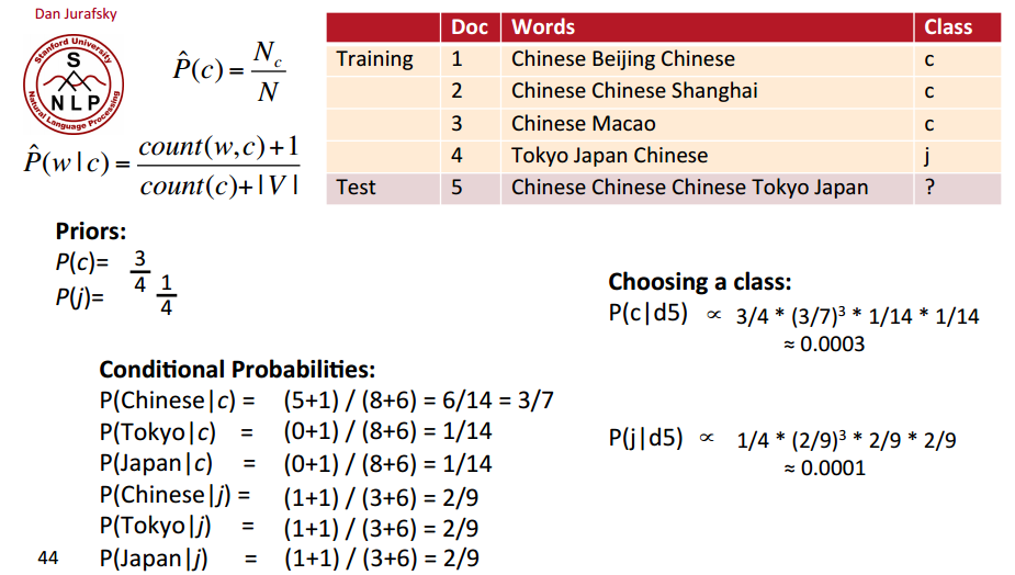
A Worked Example [Dan Jurafsky]